Read in Only First Few Rows of Data in R
Working with tabular data in R
Learning Objectives
- Load external data from a .csv file into a data frame in R with
read.csv()- Find basic properties of a data frames including size, course or type of the columns, names of rows and columns by using
str(),nrow(),ncol(),dim(),length(),colnames(),rownames()- Apply
head()andtail()to inspect rows of a data frame.- Generate summary statistics for a data frame
- Use indexing to select rows and columns
- Apply logical conditions to select rows and columns
- Add together columns and rows to a data frame
- Manipulate categorical data with
factors,levels()andas.character()- Modify how character strings are handled in a data frame.
- Format dates in R and summate time differences
- Apply
df$new_col <- new_colto add together a new column to a information frame.- Use
cbind()to add a new column to a information frame.- Use
rbind()to add a new row to a data frame.- Use
na.omit()to remove rows from a data frame withNAvalues.
## Loading tabular information
I the most common ways of getting information into R is to read in a table. And – you lot guessed it – we read it into a data frame! We will take a uncomplicated CSV file as case. What is a CSV file?
You lot may know about the Stanford Open Policing Project and we volition be working with a sample dataset from their repository (https://openpolicing.stanford.edu/information/). The sample I extracted contains information about traffic stops for black and white drivers in the country of Mississippi during Jan 2013 to mid-July of 2016.
We are going to use the R function download.file() to download the CSV file that contains the traffic stop information, and nosotros volition use read.csv() to load into memory the content of the CSV file equally an object of class data.frame.
To download the data into your local information/ subdirectory, run the following:
You are now ready to load the information:
This statement doesn't produce any output because, as you might recall, assignments don't brandish annihilation. If we desire to bank check that our information has been loaded, nosotros can print the variable's value: trafficstops.
Wow… that was a lot of output. At to the lowest degree it means the information loaded properly. Allow'southward bank check the height (the first 6 lines) of this data frame using the role head():
#> id land stop_date county_name county_fips #> i MS-2013-00001 MS 2013-01-01 Jones County 28067 #> 2 MS-2013-00002 MS 2013-01-01 Lauderdale County 28075 #> 3 MS-2013-00003 MS 2013-01-01 Expressway County 28113 #> iv MS-2013-00004 MS 2013-01-01 Hancock County 28045 #> 5 MS-2013-00005 MS 2013-01-01 Holmes County 28051 #> half dozen MS-2013-00006 MS 2013-01-01 Jackson County 28059 #> police_department driver_gender driver_birthdate driver_race #> 1 Mississippi Highway Patrol M 1950-06-14 Black #> two Mississippi Highway Patrol M 1967-04-06 Blackness #> 3 Mississippi Highway Patrol One thousand 1974-04-15 Blackness #> iv Mississippi Highway Patrol G 1981-03-23 White #> 5 Mississippi Highway Patrol K 1992-08-03 White #> 6 Mississippi Highway Patrol F 1960-05-02 White #> violation_raw officer_id #> ane Seat belt not used properly as required J042 #> 2 Careless driving B026 #> iii Speeding - Regulated or posted speed limit and bodily speed M009 #> iv Speeding - Regulated or posted speed limit and actual speed K035 #> 5 Speeding - Regulated or posted speed limit and actual speed D028 #> 6 Speeding - Regulated or posted speed limit and actual speed K023 Inspecting data.frame Objects
As you may recall, a data frame in R is a special case of a list, and a representation of data where the columns are vectors that all take the same length. Because the columns are vectors, they all contain the aforementioned blazon of data (e.g., characters, integers, factors, etc.).
Nosotros tin can meet this when inspecting the structure of a information frame with the function str():
#> 'data.frame': 211211 obs. of xi variables: #> $ id : chr "MS-2013-00001" "MS-2013-00002" "MS-2013-00003" "MS-2013-00004" ... #> $ country : chr "MS" "MS" "MS" "MS" ... #> $ stop_date : chr "2013-01-01" "2013-01-01" "2013-01-01" "2013-01-01" ... #> $ county_name : chr "Jones County" "Lauderdale County" "Pike County" "Hancock County" ... #> $ county_fips : int 28067 28075 28113 28045 28051 28059 28059 28043 28051 28051 ... #> $ police_department: chr "Mississippi Highway Patrol" "Mississippi Highway Patrol" "Mississippi Highway Patrol" "Mississippi Highway Patrol" ... #> $ driver_gender : chr "M" "One thousand" "G" "M" ... #> $ driver_birthdate : chr "1950-06-14" "1967-04-06" "1974-04-xv" "1981-03-23" ... #> $ driver_race : chr "Black" "Blackness" "Black" "White" ... #> $ violation_raw : chr "Seat belt non used properly as required" "Careless driving" "Speeding - Regulated or posted speed limit and actual speed" "Speeding - Regulated or posted speed limit and actual speed" ... #> $ officer_id : chr "J042" "B026" "M009" "K035" ... We already saw how the functions caput() and str() tin be useful to check the content and the construction of a data frame. Here is a non-exhaustive list of functions to go a sense of the content/construction of the data. Let's effort them out!
- Size:
-
dim(trafficstops)- returns a vector with the number of rows in the outset element, and the number of columns equally the 2d element (the dimensions of the object) -
nrow(trafficstops)- returns the number of rows -
ncol(trafficstops)- returns the number of columns -
length(trafficstops)- returns number of columns
-
- Content:
-
caput(trafficstops)- shows the first half-dozen rows -
tail(trafficstops)- shows the last half dozen rows
-
- Names:
-
names(trafficstops)- returns the column names (synonym ofcolnames()fordata.frameobjects) -
rownames(trafficstops)- returns the row names
-
- Summary:
-
str(trafficstops)- construction of the object and information about the class, length and content of each column -
summary(trafficstops)- summary statistics for each column
-
Note: almost of these functions are "generic", they tin can be used on other types of objects likewise data.frame.
Challenge
Based on the output of
str(trafficstops), can you answer the following questions?
- What is the form of the object
trafficstops?- How many rows and how many columns are in this object?
- How many counties have been recorded in this dataset?
Indexing and subsetting data frames
Our trafficstops data frame has rows and columns (information technology has 2 dimensions), if we want to excerpt some specific data from it, nosotros need to specify the "coordinates" nosotros want from it. Row numbers come outset, followed by cavalcade numbers. Withal, note that different ways of specifying these coordinates atomic number 82 to results with different classes.
trafficstops[i, 1] # first chemical element in the first column of the data frame (every bit a vector) trafficstops[1, 6] # get-go element in the 6th cavalcade (as a vector) trafficstops[, 1] # first cavalcade in the data frame (as a vector) trafficstops[1] # first column in the data frame (as a information.frame) trafficstops[1 : 3, 7] # beginning three elements in the seventh column (equally a vector) trafficstops[3, ] # the third row (as a information.frame) trafficstops[1 : 6, ] # the 1st to 6th rows, equivalent to head(trafficstops) trafficstops[, -1] # the whole data frame, excluding the first column trafficstops[- c(7 : 211211),] # equivalent to head(trafficstops) As well as using numeric values to subset a information.frame (or matrix), columns tin can exist called by name, using one of the four post-obit notations:
For our purposes, the last three notations are equivalent. RStudio knows nearly the columns in your data frame, so you can take advantage of the autocompletion feature to get the full and correct column name.
Claiming
Create a
data.frame(trafficstops_200) containing merely the observations from row 200 of thetrafficstopsdataset.Notice how
nrow()gave y'all the number of rows in ainformation.frame?
- Use that number to pull out just that last row in the data frame.
- Compare that with what you see as the final row using
tail()to make sure it's meeting expectations.- Pull out that last row using
nrow()instead of the row number.- Create a new data frame object (
trafficstops_last) from that last row.Apply
nrow()to extract the row that is in the middle of the information frame. Shop the content of this row in an object namedtrafficstops_middle.Combine
nrow()with the-note above to reproduce the beliefs ofcaput(trafficstops)keeping just the first through 6th rows of the trafficstops dataset.
## Conditional subsetting
Oftentimes times we demand to extract a subset of a data frame based on certain conditions. For example, if we wanted to wait at traffic stops in Webster County only we could say:
This is also a possibility (but slower):
#> [one] 156 #> #> Black White #> 59 97 These commands are from the R base package. In the R Data Wrangling workshop we volition talk over a different way of subsetting using functions from the tidyverse package.
Challenge
- Utilise subsetting to extract trafficstops in Hancock, Harrison, and Jackson Counties into a separate data frame
coastal_counties.- Using
coastal_counties, count the number of Black and White drivers in the three counties.- Bonus: How does the ratio of Blackness to White stops in the 3 coastal counties compare to the same ratio for stops in the entire state of Mississippi?
## Adding and removing rows and columns
To add together a new column to the data frame nosotros can utilize the cbind() part.
#> id state stop_date county_name county_fips #> i MS-2013-00001 MS 2013-01-01 Jones County 28067 #> 2 MS-2013-00002 MS 2013-01-01 Lauderdale County 28075 #> iii MS-2013-00003 MS 2013-01-01 Pike County 28113 #> 4 MS-2013-00004 MS 2013-01-01 Hancock County 28045 #> v MS-2013-00005 MS 2013-01-01 Holmes County 28051 #> 6 MS-2013-00006 MS 2013-01-01 Jackson County 28059 #> police_department driver_gender driver_birthdate driver_race #> one Mississippi Highway Patrol M 1950-06-14 Blackness #> 2 Mississippi Highway Patrol M 1967-04-06 Black #> 3 Mississippi Highway Patrol M 1974-04-xv Black #> 4 Mississippi Highway Patrol M 1981-03-23 White #> 5 Mississippi Highway Patrol M 1992-08-03 White #> 6 Mississippi Highway Patrol F 1960-05-02 White #> violation_raw officer_id #> 1 Seat belt not used properly as required J042 #> 2 Careless driving B026 #> iii Speeding - Regulated or posted speed limit and actual speed M009 #> 4 Speeding - Regulated or posted speed limit and actual speed K035 #> 5 Speeding - Regulated or posted speed limit and actual speed D028 #> half dozen Speeding - Regulated or posted speed limit and actual speed K023 #> new_col #> 1 i #> ii 2 #> three 3 #> 4 4 #> v 5 #> half dozen half dozen Alternatively, we tin also add a new column adding the new column name after the $ sign then assigning the value, similar below. Notation that this will alter the original data frame, which yous may not always desire to practice.
At that place is an equivalent role, rbind() to add a new row to a data frame. I utilise this far less ofttimes than the cavalcade equivalent. The ane thing to keep in mind is that the row to exist added to the data frame needs to match the gild and type of columns in the information frame. Recall that R's way to store multiple different data types in ane object is a listing. So if we wanted to add a new row to trafficstops we would say:
new_row <- data.frame(id= "MS-2017-12345", state= "MS", stop_date= "2017-08-24", county_name= "Tallahatchie County", county_fips= 12345, police_department= "MSHP", driver_gender= "F", driver_birthdate= "1999-06-fourteen", driver_race= "Hispanic", violation_raw= "Speeding", officer_id= "ABCD") trafficstops_withnewrow <- rbind(trafficstops, new_row) tail(trafficstops_withnewrow) #> id state stop_date county_name county_fips #> 211207 MS-2016-24293 MS 2016-07-09 George County 28039 #> 211208 MS-2016-24294 MS 2016-07-10 Copiah County 28029 #> 211209 MS-2016-24295 MS 2016-07-xi Grenada Canton 28043 #> 211210 MS-2016-24296 MS 2016-07-14 Copiah County 28029 #> 211211 MS-2016-24297 MS 2016-07-14 Copiah County 28029 #> 211212 MS-2017-12345 MS 2017-08-24 Tallahatchie Canton 12345 #> police_department driver_gender driver_birthdate driver_race #> 211207 Mississippi Highway Patrol M 1992-07-14 White #> 211208 Mississippi Highway Patrol M 1975-12-23 Black #> 211209 Mississippi Highway Patrol 1000 1998-02-02 White #> 211210 Mississippi Highway Patrol F 1970-06-14 White #> 211211 Mississippi Highway Patrol M 1948-03-11 White #> 211212 MSHP F 1999-06-xiv Hispanic #> violation_raw officer_id #> 211207 Speeding - Regulated or posted speed limit and actual speed K025 #> 211208 Speeding - Regulated or posted speed limit and actual speed C033 #> 211209 Seat belt not used properly as required D014 #> 211210 Expired or no non-commercial driver license or permit C015 #> 211211 Seat belt not used properly as required C015 #> 211212 Speeding ABCD A convenient role to know about is na.omit(). It volition remove all rows from a information frame that have at least one cavalcade with NA values.
Challenge
- Given the post-obit data frame:
What would you wait the following commands to return?
Categorical data: factors
Factors are very useful and are actually something that make R particularly well suited to working with information, so we're going to spend a little time introducing them.
Factors are used to represent chiselled data. Factors can be ordered or unordered, and understanding them is necessary for statistical analysis and for plotting.
Factors are stored as integers, and take labels (text) associated with these unique integers. While factors look (and often behave) like character vectors, they are actually integers under the hood, and you need to be careful when treating them like strings.
Once created, factors can but comprise a pre-defined set of values, known as levels. By default, R always sorts levels in alphabetical order. For instance, if you have a factor with 2 levels:
R will assign ane to the level "democrat" and two to the level "republican" (because d comes before r, even though the first element in this vector is "republican"). You lot tin can bank check this by using the function levels(), and check the number of levels using nlevels():
Sometimes, the order of the factors does not matter, other times you might want to specify the order considering it is meaningful (due east.g., "low", "medium", "high"), it improves your visualization, or it is required by a particular type of analysis. Here, one mode to reorder our levels in the party vector would exist:
#> [ane] republican democrat democrat republican #> Levels: democrat republican #> [1] republican democrat democrat republican #> Levels: republican democrat In R'due south retentivity, these factors are represented by integers (1, 2, 3), simply are more informative than integers because factors are self describing: "democrat", "republican" is more than descriptive than ane, 2. Which one is "republican"? You lot wouldn't be able to tell simply from the integer data. Factors, on the other hand, have this data built in. It is especially helpful when there are many levels (like the canton names in our example dataset).
Converting factors
If yous need to convert a factor to a character vector, you lot use as.character(x).
Converting factors where the levels appear as numbers (such every bit concentration levels, or years) to a numeric vector is a little trickier. One method is to convert factors to characters and then numbers. Another method is to use the levels() function. Compare:
Detect that in the levels() approach, 3 important steps occur:
- We obtain all the cistron levels using
levels(f) - We convert these levels to numeric values using
equally.numeric(levels(f)) - We then access these numeric values using the underlying integers of the vector
fas indices inside the square brackets
Renaming factors
When your data is stored as a cistron, you lot can utilise the plot() function to become a quick glance at the number of observations represented by each factor level. Permit's look at the number of blacks and whites in the dataset:
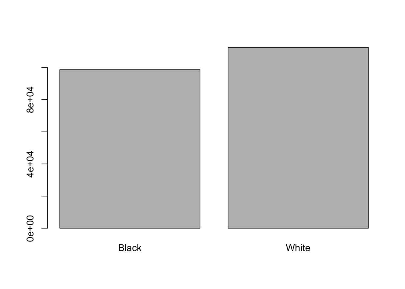
In that location seem to exist a number of individuals for which the race information hasn't been recorded.
Additionally, for these individuals, there is no label to bespeak that the data is missing. Let's rename this characterization to something more meaningful. Before doing that, we're going to pull out the data on race and work with that data, and then we're not modifying the working re-create of the information frame:
#> [1] Black Black Blackness White White White #> Levels: Black White #> [ane] "" "Black" "White" #> [one] "Missing" "Black" "White" #> [1] Blackness Blackness Black White White White #> Levels: Missing Black White Claiming
- Rename "Blackness" to "African American".
- Now that nosotros have renamed the factor level to "Missing", tin you recreate the barplot such that "Missing" is concluding (to the right)?
Using stringsAsFactors
By default, when edifice or importing a data frame with read.csv(), the columns that contain characters (i.east., text) are read as such. (This was introduced in R Version 4.) Depending on what you intend to do with the data, you may want to continue these columns as character or catechumen to gene. To exercise so, read.csv() and read.table() have an argument called stringsAsFactors which tin exist set up to TRUE.
Claiming
Can you predict the form for each of the columns in the following example? Check your guesses using
str(country_climate): * Are they what you expected? Why? Why not? * What would accept been different if nosotros had addedstringsAsFactors = FALSEto this telephone call? * What would you need to modify to ensure that each column had the accurate data blazon?``` country_climate <- information.frame( country=c("Canada", "Panama", "South Africa", "Commonwealth of australia"), climate=c("cold", "hot", "temperate", "hot/temperate"), temperature=c(10, 30, 18, "xv"), northern_hemisphere=c(Truthful, Truthful, Simulated, "FALSE"), has_kangaroo=c(Imitation, FALSE, FALSE, 1) ) ```
The automatic conversion of data type is sometimes a approving, sometimes an annoyance. Be aware that it exists, learn the rules, and double check that data you import in R are of the right type within your data frame. If not, apply it to your reward to detect mistakes that might have been introduced during data entry (a letter of the alphabet in a column that should but comprise numbers for example).
Dates
I of the most mutual bug that new (and experienced!) R users take is converting engagement and fourth dimension data into a variable that is appropriate and usable during analyses. If you lot have control over your information information technology might be useful to ensure that each component of your engagement is stored as a separate variable, i.east a split column for 24-hour interval, calendar month, and year. However, often we do non accept command and the appointment is stored in ane single column and with varying order and separating characters betwixt its components.
Using str(), we can come across that both dates in our data frame stop_date and driver_birthdate are each stored in one column.
Every bit an example for how to piece of work with dates let united states see if in that location are seasonal differences in the number of traffic stops.
We're going to be using the ymd() function from the bundle lubridate . This function is designed to take a vector representing year, calendar month, and solar day and convert that information to a POSIXct vector. POSIXct is a class of data recognized by R as being a date or appointment and time. The argument that the function requires is relatively flexible, but, as a all-time practice, is a character vector formatted as "YYYY-MM-DD".
Outset past loading the required bundle:
The ymd office likewise has nicely taken care of the fact that the original format of the date cavalcade is a factor!
We tin at present easily extract year, month, and date using the respective functions: year(), calendar month(), and day() similar so:
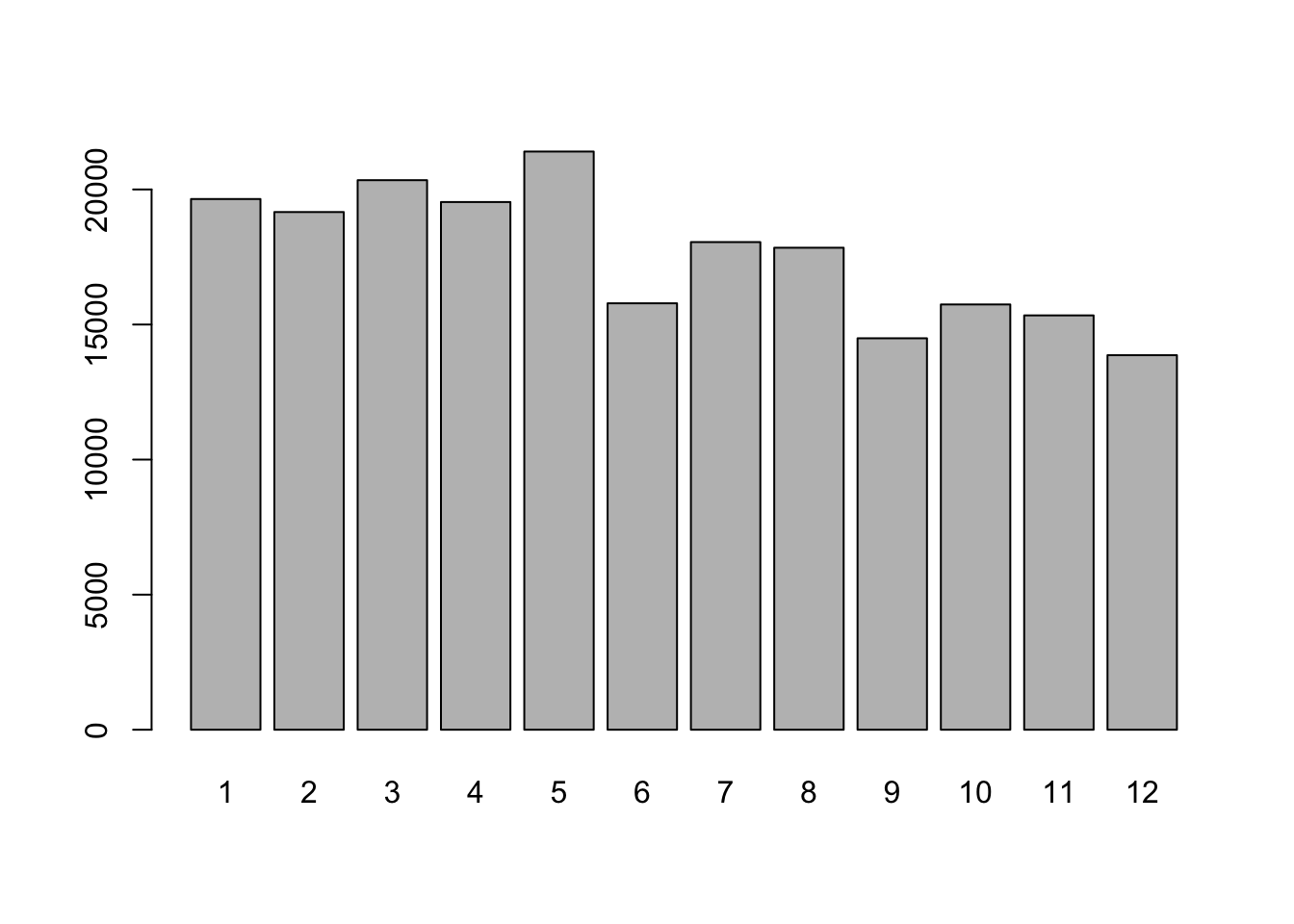
Challenge
- Are there more stops in certain months of the year or certain days of the month?
Challenge
- Determine the age of the driver in years (guess) at the fourth dimension of the stop:
- Extract
driver_birthdateinto a vectorbirth_date- Create a new vector
agewith the driver's age at the time of the terminate in years- Coerce
ageto a factor and use theplotpart to check your results. What practise you discover?
Source: https://cengel.github.io/R-intro/data.html
0 Response to "Read in Only First Few Rows of Data in R"
Postar um comentário